Lab 10: Localization(sim)

PRE-LAB:

I followed the instructions provided in the Simulation tool—installing all dependencies, the appropriate wheel file for my OS and Python version, and the Box2D library. Using the GUI, I explored various commands to observe how the robot would respond. I used Open Loop Control to navigate the robot through the space and observed that movement commands continued indefinitely unless explicitly counteracted by an opposing command. Below is a plot comparing the robot’s odometry with the ground truth for the trajectory I created.

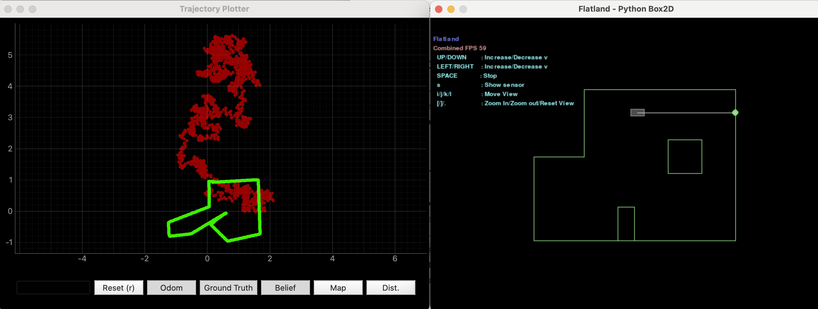
Analyzing the odometry plot (the red dots) it does not look accurate at all. However, the ground truth plot (green dots) seem accurate with just a few undershooting angles in a few turns.

TASKS:

The following function were written to run the Bayes Filter.

COMPUTE CONTROL:

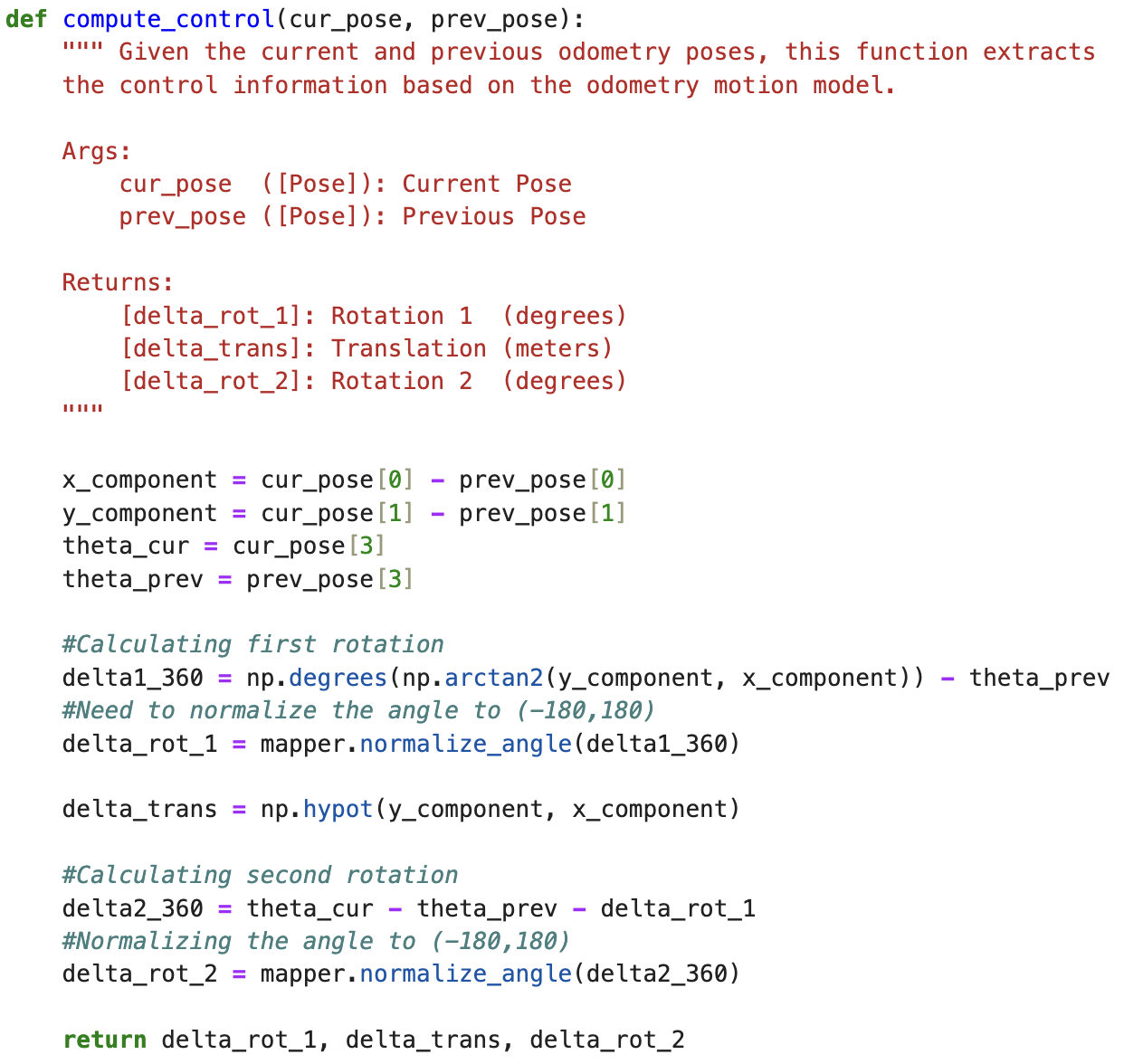
The compute_control() function calculates the first rotation, translation, and second rotation by using the robot’s current pose and previous pose as inputs. The equations used for these calculations are shown below (from Lecture 18).

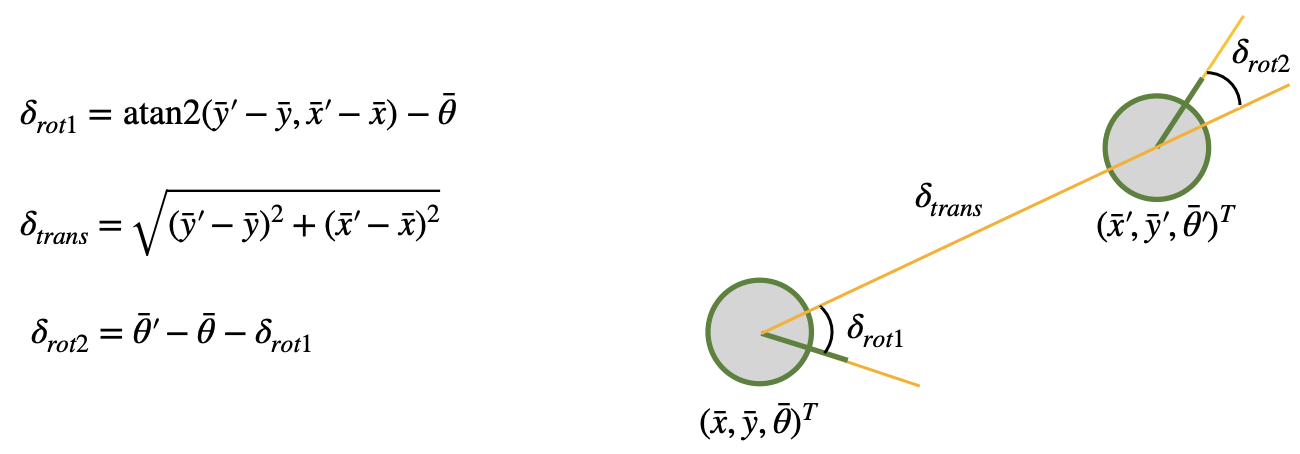
To simplify the equations in Pyhton, I created a variable called x_component to store the difference between the x-coordinates of the current and previous poses. I did the same for the y-coordinates.

ODOMETRY MOTION MODEL:

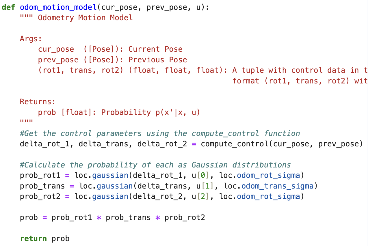
The odom_motion_model() function also takes in the current pose and previous pose, but it additionally considers the odometry control input. It uses the parameters calculated by the compute_control() function and estimates the probability that the robot reached its current position given the previous pose. These probabilities are modeled using a Gaussian distribution.

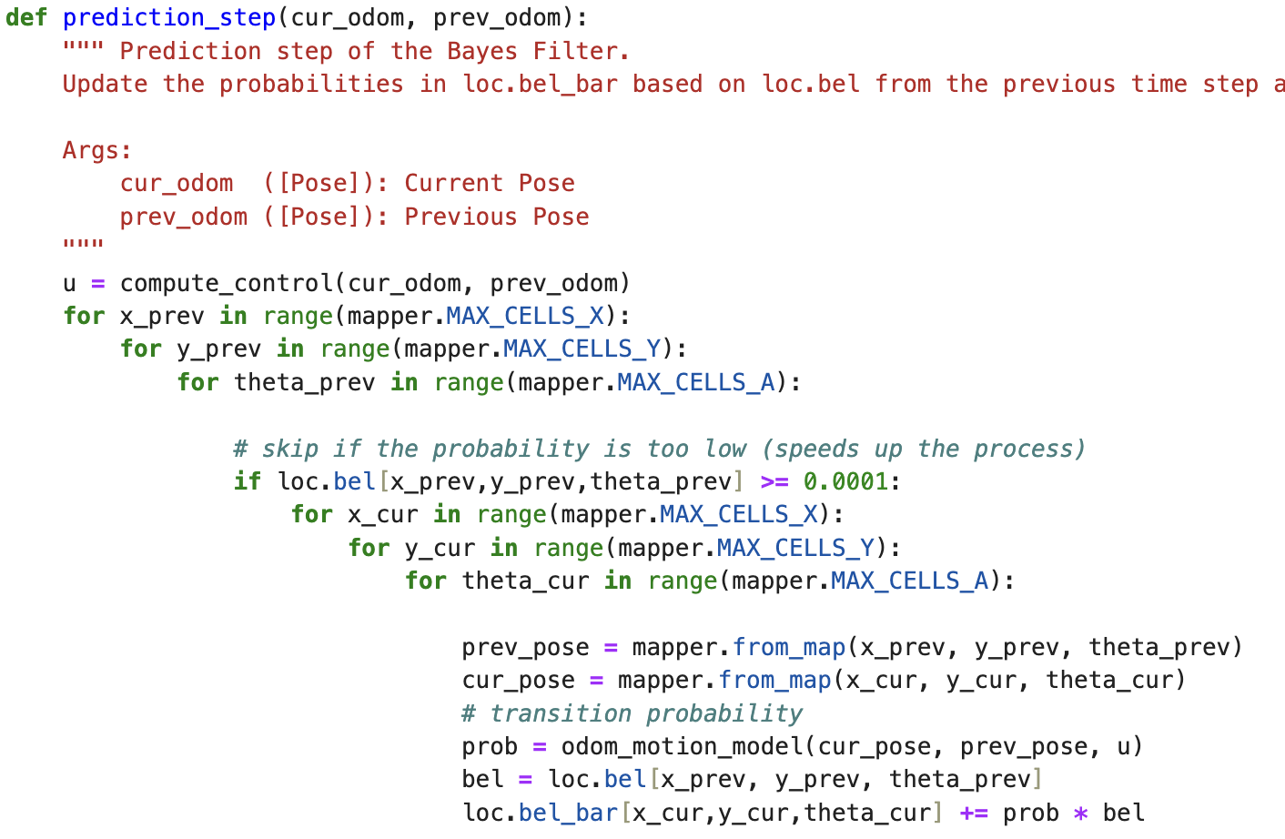
PREDICTION STEP:

The prediction_step() function calculates the probability that the robot is in each cell of the grid. It does this by taking the current and previous poses and iterating through the entire grid to compute a predicted belief using the odom_motion_model() function.

To reduce computational load, the function skips calculations for cells where the probability drops below 0.0001, since the likelihood of the robot being in those cells is very low. While this speeds up the process, it can slightly reduce the precision and accuracy of the filter.

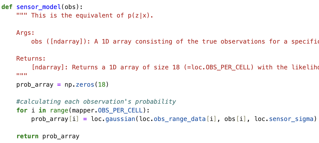
SENSOR MODEL:

The sensor_model() function calculates the probability of each input observation occurring in the current state, modeling them with a Gaussian distribution. It returns a 1D array of the same size as the input, where each element represents the corresponding probability.

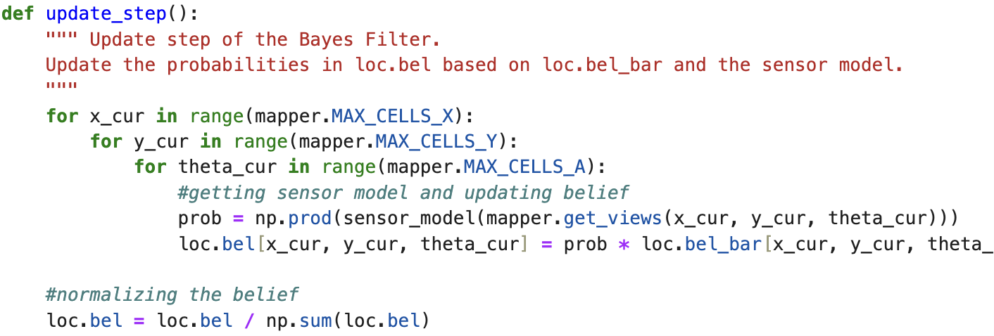
UPDATE STEP:

And finally, the update_step() function iterates through all the cells in the grid, gets the probability at each cell using sensor_model(), and then updates the belief by multiplying this probability with the predicted belief. The resulting values are then normalized.

SIMULATION RESULTS:

Here is my succesful run of the Bayes Filter simulation. It ran for 15 iterations, which can be seen below.

And this is the final plot for this run:

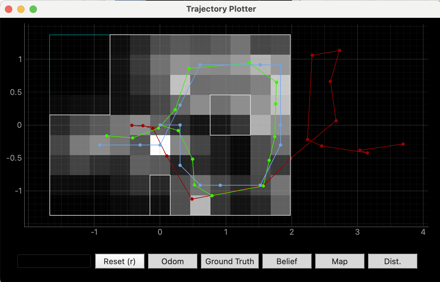
The red line represents the odometry measurements, the green line is the ground truth, and the blue line shows the belief. The different shades of grid cells indicate the strength of the belief—lighter cells represent higher belief values.

You can see how the ground truth and belief follow very similar paths, which is good. The probability however seems to be pretty noisy and not precise. Which I may need to consider when uploading the Bayes filter rto my robot for the next lab.

Overall, I think the Bayes filter would perform reasonably well on the robot, but it may require a second set of data to validate the results, as the filter appears to be a bit noisy.

REFERENCES:

For this lab I referenced, Stephan Wagner's and Mikayla Lahr's labs from previous years. I also used ChatGPT to help with the grammar.